Why?

June 7, 2017

Security: the dangers of copying and pasting R code

Filed under: Computing, R — Tags: — csgillespie @ 10:11 am

Most of the time when we stumble across a code snippet online, we often blindly copy and paste it into the R console. I suspect almost everyone does this. After all, what’s the harm? Consider this simple piece of R code that performs simple linear regression

# Generate data
x = rnorm(10)
y = rnorm(10)
message(“All your base are belong to us.”)
# Simple linear regression 
m = lm(y ~ x)

Now highlight the above piece of R code and copy and paste it into your console; look carefully at what you’ve pasted. A new line has magically appeared.

# Generate data
x = rnorm(10)
y = rnorm(10)
message("All your base are belong to us.")
# Simple linear regression
m = lm(y ~ x)

Due to some sneaky CSS magic, I was able to hide the message() statement. If I was evil, I could have changed this to a system, source, or any other command.

The CSS code simply sets the message() function to the background color, changes the font size and makes it un-selectable (see this post for details).

So remember, be careful with your copy and pasting!

January 22, 2017

Input/output benchmarks

Filed under: Computing, R — Tags: — csgillespie @ 5:08 pm

To quantify the impact of the CPU on an analysis, I created the package benchmarkme. The idea is simple. If everyone runs the same R script, we can easily compare machines.

One of the benchmarks in the package is for comparing read/write speeds; we write a large CSV file (using write.csv) and read it back in using read.csv

The package is on CRAN can be installed in the usual way

install.packages("benchmarkme")

Running

library(benchmarkme)
## If your computer is relatively slow, remove 200 from below
res = benchmark_io(runs = 3, size = c(5, 50, 200))
## Upload you data set
upload_results(res)

creates three matrices of size 5MB, 20MB and 200MB, writes the associated CSV file to the directory

Sys.getenv("TMPDIR")

and then reads the data set back into R. The object res contains the timings which can compared to other users via

plot(res)

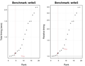
rplot01

The above graph plots the current benchmarking results for writing a 5MB file (my machine is relatively fast).

Shiny

You can also compare your results using the Shiny interface. Simply create a results bundle

 create_bundle(res, filename = "results.rds")

and upload to the webpage.

Network drives

Often the dataset we wish to access is on a network drive. Unfortunately, network drives can be slow. The benchmark_io function has an argument that allows us to change the directory and estimate the network drive impact

res_net = benchmark_io(runs = 3, size = c(5, 20, 200), 
                           tmpdir = "path_to_dir")


January 9, 2017

benchmarkme Update

Filed under: Computing, R — Tags: , — csgillespie @ 8:36 pm

When discussing how to speed up slow R code, my first question is what is your computer spec? It always surprises me when complex biological experiments, costing a significant amount of money, are analysed using a six year old laptop. A new desktop machine costs around £1000 and that money would be saved within a month in user time. Typically the more the RAM you have, the larger the dataset you can handle. However it’s not so obvious of the benefit of upgrading the processor.

To quantify the impact of the CPU on an analysis, I created the package benchmarkme. The aim of this package is to provide a set of benchmarks routines and data from past runs. You can then compare your machine, with other CPUs.

The package is now on CRAN and can be installed in the usual way

install.packages("benchmarkme")

The benchmark_std() function assesses numerical operations such as loops and matrix operations. This benchmark comprises of three separate benchmarks: prog, matrix_fun, and matrix_cal. If you have less than 3GB of RAM (run `get_ram()` to find out how much is available on your system), then you should kill any memory hungry applications, e.g. firefox, and set `runs = 1` as an argument.

To benchmark your system, use

library("benchmarkme")
res = benchmark_std(runs = 3)

You can compare your results to other users via

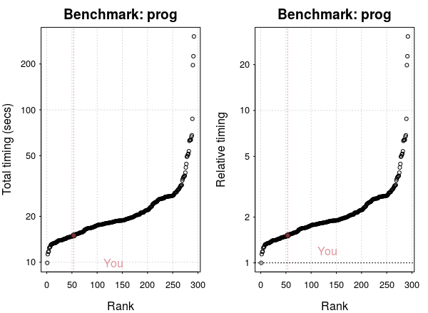
plot(res)


My laptop is ranked around 50 out of 300. However, relative to the fastest processor, there’s not much difference.

Finally upload your results for the benefit of other users

## You can control exactly what is uploaded. See details below.
upload_results(res)

Shiny

You can also compare your results using the Shiny interface. Simply create a results bundle

 create_bundle(res, filename = "results.rds")

and upload to the webpage.

What’s uploaded

Two objects are uploaded:

1. Your benchmarks from benchmark_std or benchmark_io;
2. A summary of your system information (get_sys_details()).

The get_sys_details() returns:

Sys.info();
get_platform_info();
get_r_version();
get_ram();
get_cpu();
get_byte_compiler();
get_linear_algebra();
installed.packages();
Sys.getlocale();
– The `benchmarkme` version number;
– Unique ID – used to extract results;
– The current date.

The function Sys.info() does include the user and nodenames. In the public release of the data, this information will be removed. If you don’t wish to upload certain information, just set the corresponding argument, i.e.

upload_results(res, args = list(sys_info=FALSE))

April 22, 2016

R Courses at Newcastle

Filed under: Computing, R, Teaching — Tags: , — csgillespie @ 7:09 pm

Over the next two months I’m running a number of R courses at Newcastle University.

  • May 2016
    • May 10th, 11th: Predictive Analytics
    • May 16th – 20th: Bioconductor
    • May 23rd, 24th: Advanced programming
  • June 2016
    • June 8th: R for Big Data
    • June 9th: Interactive graphics with Shiny

Since these courses are on  advanced topics, numbers are limited (there’s only a couple of places left on Predictive Analytics). If you are interested in attending, sign up as soon as possible.

Getting to Newcastle is easy. The airport is 10 minutes from the city centre and has direct flights to the main airport hubs: Schiphol, Heathrow, and Paris.  The courses at Newcastle attract participants from around the world; at the April course, we had representatives from North America, Sweden, Germany,  Romania and Geneva.

Cost: The courses cost around £130 per day (more than half the price of certain London courses!)


Onsite courses available on request.

April 1, 2016

RStudio addins manager

Filed under: Computing, R — Tags: — csgillespie @ 12:36 am

RStudio addins let you execute a bit of R code or a Shiny app through the RStudio IDE, either via the Addins dropdown menu or with a keyboard shortcut. This package is an RStudio addin for managing other addins. To run these addins, you need the latest version of RStudio.

Installation

The package can be installed via devtools

## Need the latest version of DT as well
devtools::install_github('rstudio/DT')
devtools::install_github("csgillespie/addinmanager")

Running addins

After installing the package, the Addins menu toolbar will be populated with a new addin called Addin Manager. When you launch this addin, a DT table will be launched:

screenshot

In the screenshot above, the highlighted addins, shinyjs and ggThemeAssit, indicate that this addins have already installed.

When you click Done

  • Highlighted addins will be installed.
  • Un-highlighted addins will be removed.

Simple!

Including your addin

Just fork and alter the addin file which is located in the inst/extdata directory of the package. This file is a csv file with three columns:

  • addin Name/title
  • Brief Description
  • Package. If the package is only on github, use name/repo.

The initial list of addins was obtain from daattali’s repo.

February 16, 2016

RANDU: The case of the bad RNG

Filed under: Computing, R — Tags: , , — csgillespie @ 12:15 pm

The German Federal Office for Information Security (BSI) has established
criteria for quality random number generator (rng):

  • A sequence of random numbers has a high probability of containing no identical consecutive elements.
  • A sequence of numbers which is indistinguishable from true random’ numbers (tested using statistical tests.
  • It should be impossible to calculate, or guess, from any given sub-sequence, any previous or future values in the sequence.
  • It should be impossible, for all practical purposes, for an attacker to calculate, or guess the values used in the random number algorithm.

Points 3 and 4 are crucial for many applications. Everytime you make a
phone call, contact to a wireless point, pay using your credit card random
numbers are used.

Designing a good random number generator is hard and as a general rule you should never try to. R comes with many good quality random generators. The default generator is the Mersenne-Twister. This rng has a huge period of 2^{19937}-1 (how many random numbers are generated before we have a repeat).

Linear congruential generators

A linear congruential generator (lcg) is a relatively simple rng (popular in the 60’s and 70’s). It has a simple form of

r_{i}=(ar_{i-1}+b) \textrm{ mod }m, \quad i=1, 2, \ldots, m

where $latexr_0$ is the initial number, known as the seed, and \(a,b,m\) are the multiplier, additive constant and modulo respectively. The parameters are all integers.

The modulo operation means that at most m different numbers can be generated
before the sequence must repeat – namely the integers 0,1,2, \ldots, m-1. The
actual number of generated numbers is h \leq m, called the period of
the generator.

The key to random number generators is in setting the parameters.

RANDU

RANDU was a lcg with parameters m=2^{31}, a=65539 and b=0. Unfortunately this is a spectacularly bad choice of
parameters. On noting that a=65,539=2^{16}+3, then

r_{i+1} = a r_i = 65539 \times r_i = (2^{16}+3)r_i \;.

So

r_{i+2} = a\;r_{i+1} = (2^{16}+3) \times r_{i+1} = (2^{16}+3)^2 r_i \;.

On expanding the square, we get

r_{i+2} = (2^{32}+6\times 2^{16} + 9)r_i = [6 (2^{16}+3)-9]r_i = 6 r_{i+1} - 9 r_i \;.

Note: all these calculations should be to the mod 2^{31}. So there is a large
correlation between the three points!

If compare randu to a standard rng (code in a gist)

Rplot1

It’s obvious that randu doesn’t produce good random numbers. Plotting  x_i, x_{i-1} and x_{i-2} in 3d

Rplot2

Generating the graphics

The code is all in a gist and can be run via


devtools::source_gist("https://gist.github.com/csgillespie/0ba4bbd8da0d1264b124")

You can then get the 3d plot via


scatterplot3d::scatterplot3d(randu[,1], randu[,2], randu[,3],
angle=154)
## Interactive version
threejs::scatterplot3js(randu[,1], randu[,2], randu[,3])

February 15, 2016

Shiny benchmarks

Filed under: Computing, R — Tags: , — csgillespie @ 5:49 pm

A couple of months ago, the first version of benchmarkme was released. Around 140 machines have now been benchmarked.

From the fastest (an Apple i7) which ran the tests in around 10 seconds, to the slowest (an Atom(TM) CPU N450 @ 1.66GHz) which took 420 seconds! Other interesting statistics:

  • Around 6% of people ran BLAS optimised versions of R;
  • No-one (except for machines that I used) ran a byte compiled version of the package.

I intend to write to a blog post or two on BLAS and byte compiling, but for the meantime you can investigate the results via the new shiny interface. The package is still only available on github and can be installed via:


## Update the package
install.packages(c("drat", "httr", "Matrix", "shiny"))
drat::addRepo("csgillespie")
install.packages("benchmarkme", type="source")

You then load the package in the usual way


library("benchmarkme")
## View past results
plot_past()
## shine() # Needs shiny
## get_datatable_past() # Needs DT

To benchmark your system, use


## This will take somewhere between 0.5 and 5 minutes
## Increase runs if you have a higher spec machine
res = benchmark_std(runs=3)

You can then compare your results other users


plot(res)
## shine(res)
## get_datatable(res)

and upload your results


## You can control exactly what is uploaded. See details below.
upload_results(res)

This function returns a unique identifier that will allow you to identify your results from the public data sets.

December 1, 2015

Crowd sourced benchmarks

Filed under: Computing, R — Tags: , — csgillespie @ 10:25 am

When discussing how to speed up slow R code, my first question is what is your computer spec? It always surprises me when complex biological experiments, costing a significant amount of money, are analysed using a six year old laptop. A new desktop machine costs around £1000 and that money would be saved within a month in user time. Typically the more the RAM you have, the larger the dataset you can handle. However it’s not so obvious of the benefit of upgrading the processor.

To quantify the impact of the CPU on an analysis, I’ve create a simple benchmarking package. The aim of this package is to provide a set of benchmarks routines and data from past runs. You can then compare your machine, with other CPUs. The package currently isn’t on CRAN, but you can install it via my drat repository

install.packages(c("drat", "httr", "Matrix"))
drat::addRepo("csgillespie")
install.packages("benchmarkme", type="source")

You can load the package in the usual way, and view past results via


library("benchmarkme")
plot_past()

to get

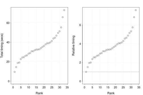
Timings1

Currently around forty machines have been benchmarked. To benchmark and compare your own system just run


## On slower machines, reduce runs.
res = benchmark_std(runs=3)
plot(res)

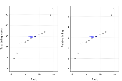
gives

my_benchmark

The final step is to upload your benchmarks


## You can control exactly what is uploaded. See the help page
upload_results(res)

The current record is held by a Intel(R) Core(TM) i7-4712MQ CPU.

July 12, 2011

Reviewing a paper that uses GPUs

Filed under: Computing, Publications — Tags: , , , , , — csgillespie @ 1:53 pm

Graphical processing units (GPUs) are all the rage these days. Most journal issues would be incomplete if at least one article didn’t mention the word “GPUs”. Like any good geek, I was initially interested with the idea of using GPUs for statistical computing. However, last summer I messed about with GPUs and  the sparkle was removed. After looking at a number of papers, it strikes me that reviewers are forgetting to ask basic questions when reviewing GPU papers.

  1. For speed comparisons, do the authors compare a GPU with a multi-core CPU. In many papers, the comparison is with a single-core CPU. If a programmer can use CUDA, they can certainly code in pthreads or openMP. Take off a factor of eight when comparing to a multi-core CPU.
  2. Since a GPU has (usually) been bought specifically for the purpose of the article, the CPU can be a few years older. So, take off a factor of two for each year of difference between a CPU and GPU.
  3. I like programming with doubles. I don’t really want to think about single precision and all the difficulties that entails. However, many CUDA programs are compiled as single precision. Take off a factor of two for double precision.
  4. When you use a GPU, you split the job in blocks of threads. The number of threads in each block depends on the type of problem under consideration and can have a massive speed impact on your problem. If your problem is something like matrix multiplication, where each thread multiplies two elements, then after a few test runs, it’s straightforward to come up with an optimal thread/block ratio. However, if each thread is a stochastic simulation, it now becomes very problem dependent. What could work for one model, could well be disastrous for another.
So in many GPU articles the speed comparisons could be reduced by a factor of 32!
Just to clarify, I’m not saying that GPUs have no future, rather, there has been some mis-selling of their potential usefulness in the (statistical) literature.

June 16, 2011

Character occurrence in passwords

Filed under: Computing, Geekery, R — Tags: , , , , , — csgillespie @ 12:52 pm

As everyone knows, it seems that Sony is taking a bit of a battering from hackers.  Thanks to Sony, numerous account and password details are now circulating on the internet. Recently, Troy Hunt carried out a brief analysis of the password structure. Here is a summary of his post:

  • There were around 40,000 passwords, of which 8000 would fail a simplistic dictionary attack;
  • Only 1% of passwords contained non-alphanumeric passwords;
  • 93% of passwords were between 6 and 10 characters.

In this post, we will investigate the remaining 32,000 passwords that passed the dictionary attack.

Distribution of characters

As Troy points out, the vast majority of passwords only contained a single type, i.e. all lower or all upper case. However, it turns out that things get even worst when we look at character frequency.

In the password database, there are a 78 unique characters. So if passwords were truly random, each character should occur with probability 1/78 = 0.013. However when we calculate the actual password occurrence, we see that it clearly isn’t random. The following figure shows the top 20 password characters, with the red line indicting 1/78.

Unsurprisingly, the vowels “e”, “a” and “o” are very popular, with the most popular numbers being 1,2, and 0 (in that order). No capital letters make it into the top twenty. We can also construct the cumulative probability plot for character occurrence. In the following figure, the red dots show the pattern we would expect if the passwords were truly random (link to a larger version of the plot):

Clearly, things aren’t as random as we would like.

Character order

Let’s now consider the order that the characters appear. To simplify things, consider only the eight character passwords. The most popular number to include in a password is “1”. If placement were random, then in passwords containing the number “1” we would expect to see the character evenly distributed. Instead, we get:

   ##Distribution of "1" over eight character passwords
   0.06 0.03 0.04 0.04 0.13 0.13 0.22 0.34

So in around of 84% of passwords that contain the number “1”, the number appears only in the second half of the password. Clearly, people like sticking a number “1” towards the end of their password.

We get a similar pattern with “2”:

   0.05 0.05 0.04 0.05 0.13 0.11 0.30 0.27

and with “!”

   #Small sample size here
   0.00 0.00 0.00 0.00 0.00 0.11 0.16 0.74

We see similar patterns with other alpha-numeric characters.

Number of characters needed to guess a password

Suppose we constructed all possible passwords using the first N most popular characters. How many passwords would that cover in our sample? The following figure shows proportion of passwords covered in our list using the first N characters:

To cover 50% of passwords in all list, we only need to use the first 27 characters. In fact, using only 20 characters covers around 25% of passwords, while using 31 characters covers 80% of passwords. Remember, these passwords passed the dictionary attack.

Summary

Typically when we calculate the probability of guessing a password, we assume that each character is equally likely to be chosen, i.e. the probability of choosing “e” is the same as choosing “Z”. This is clearly false. Also, since many systems now force people to have different character types in their password, it is too easy for users just to tack on a number as their final digit. I don’t want to go into how to efficiently explore “password space”, but it’s clear that a brute force search isn’t the way to go.

Personally, I’ve abandoned trying to remember passwords a long time ago, and just use a password manager. For example, my wordpress password is over 12 characters and consists of a completely random mixture of alphanumeric and special characters. Of course, you just need to make sure your password manager is secure….

Older Posts »

Blog at WordPress.com.