Random variable generation (Pt 3 of 3)

Ratio-of-uniforms

This post is based on chapter 1.4.3 of Advanced Markov Chain Monte Carlo.  Previous posts on this book can be found via the  AMCMC tag.

The ratio-of-uniforms was initially developed by Kinderman and Monahan (1977) and can be used for generating random numbers from many standard distributions. Essentially we transform the random variable of interest, then use a rejection method.

The algorithm is as follows:

Repeat until a value is obtained from step 2.

1. Generate uniformly over .
2. If . return as the desired deviate.

The uniform region is

In AMCMC they give some R code for generate random numbers from the Gamma distribution.

I was going to include some R code with this post, but I found this set of questions and solutions that cover most things. Another useful page is this online book.

Thoughts on the Chapter 1

The first chapter is fairly standard. It briefly describes some results that should be background knowledge. However, I did spot a few a typos in this chapter. In particular when describing the acceptance-rejection method, the authors alternate between and .

Another downside is that the R code for the ratio of uniforms is presented in an optimised version. For example, the authors use EXP1 = exp(1) as a global constant. I think for illustration purposes a simplified, more illustrative example would have been better.

This book review has been going with glacial speed. Therefore in future, rather than going through section by section, I will just give an overview of the chapter.

Random variable generation (Pt 2 of 3)

Acceptance-rejection methods

This post is based on chapter 1.4 of Advanced Markov Chain Monte Carlo.

Another method of generating random variates from distributions is to use acceptance-rejection methods. Basically to generate a random number from , we generate a RN from an envelope distribution , where .  The acceptance-rejection algorithm is as follows:

Repeat until we generate a value from step 2:

1. Generate from and from

2. If , return (as a random deviate from ).

Example: the standard normal distribution

This example illustrates how we generate RNs using the logistic distribution as an envelope distribution. First, note that

On setting , we get . This method is fairly efficient and has an acceptance rate of

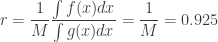
since both and are normalised densities.

R code

This example is straightforward to code:

myrnorm = function(M){
  while(1){
    u = runif(1); x = rlogis(1, scale = 0.648)
    if(u < dnorm(x)/M/dlogis(x, scale = 0.648))
      return(x)
  }
}

To check the results, we could call myrnorm a few thousand times:

hist(replicate(10000, myrnorm(1.1)), freq=FALSE)
lines(seq(-3, 3, 0.01), dnorm(seq(-3, 3, 0.01)), col=2)

Example: the standard normal distribution with a squeeze

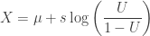
Suppose the density is expensive to evaluate. In this scenario we can employ an easy to compute function , where . is called a squeeze function. In this example, we’ll use a simple rectangular function, where for . This is shown in the following figure:

The modified algorithm is as follows:

Repeat until we generate a value from step 2:

1. Generate from and from

2. If or , return (as a random deviate from ).

Hence, when we don’t have to compute . Obviously, in this example isn’t that difficult to compute.

Random variable generation (Pt 1 of 3)

As I mentioned in a recent post, I’ve just received a copy of Advanced Markov Chain Monte Carlo Methods. Chapter 1.4 in the book (very quickly) covers random variable generation.

Inverse CDF Method

A standard algorithm for generating random numbers is the inverse cdf method. The continuous version of the algorithm is as follows:

1. Generate a uniform random variable

2. Compute and return

where is the inverse of the CDF. Well known examples of this method are the exponential distribution and the Box-Muller transform.

Example: Logistic distribution

I teach this algorithm in one of my classes and I’m always on the look-out for new examples. Something that escaped my notice is that it is easy to generate RN’s using this technique from the Logistic distribution. This distribution has CDF

and so we can generate a random number from the logistic distribution using the following formula:

Which is easily converted to R code:

myRLogistic = function(mu, s){
  u = runif(1)
  return(mu + s log(u/(1-u)))
}

Advanced Markov Chain Monte Carlo Methods (AMCMC)

I’ve just received my copy of Advanced Markov Chain Monte Carlo Methods, by Liang, Liu, & Carroll. Although my PhD didn’t really involve any Bayesian methodology (and my undergrad was devoid of any Bayesian influence), I’ve found that the sort of problems I’m now tackling in systems biology demand a Bayesian/MCMC approach. There are a number of introductory books on MCMC, but not that many on advanced techniques.

This book suggests that it could be used as a possible textbook or reference guide in a one-semester statistics graduate course. I’m not entirely convinced that it would be a good textbook, but as a reference it looks very promising. A word of warning, if you’re not familiar with MCMC then you should try the Dani Gamerman MCMC book first. Some later chapters look particularly interesting, including topics on adaptive proposals, population-based MCMC methods and dynamic weightings.

Anyway, I intend to work through the book (well at least a few of the chapters) and post my results/code as I go. Well that’s the plan anyway.